
BRIFS Forecasts
|
Forecast date selection
Videos are only displayed in Google Chrome, Mozilla Firefox and Opera. |
Selected day:
|
BRIFS Rissaga warning levels in Ciutadella The figure above shows the results of all available BRIFS simulations computed in the previous 48 hours (the darker the pointer, the more recent the prediction). Each 6-hour time slot contains a variable number of predictions, from 1 to 4, according to availability. Intermediate predictions starting at 12:00 UTC are only performed when high-frequency atmospheric perturbations are detected in the WRF simulation. |
|
Sea level anomaly predictions Sea level anomalies are displayed at three locations: 1) in Ciutadella harbour, 2) "off Ciutadella" (i.e. over the shelf at the entrance of Ciutadella inlet), and 3) in the middle of the Menorca Channel. The position of these three locations is indicated in the figure BRIFS domain configuration. |
| 0-24h prediction | 24-48h prediction |
|---|---|
| Download video | Download video |
|
Atmospheric sea level pressure evolution at P1, P2, P3, P4, P5 and P6 |
Atmospheric sea level pressure evolution at P7, P8, P9, P10, P11 and P12 |
BRIFS General Description
|
The Balearic RIssaga Forecasting System (BRIFS) aims to quantitatively predict the occurrence of extreme sea level oscillations associated with meteotsunamis in the Menorcan harbour of Ciutadella. Combining both atmospheric and oceanic high-resolution modelling, the system provides 48-hour predictions of air pressure disturbances and associated sea level response over the Balearic shelf and in Ciutadella harbour. The system is run twice a day when high-resolution atmospheric pressure oscillations are detected, once a day otherwise. |
BRIFS Configuration
|
The Weather Research and Forecasting model (WRF) is implemented in a two-nested-grid configuration over the Western Mediterranean basin, with a grid refinement (4km) over an area around the Balearic Islands extending to the South until the Algerian coast. Ninety-seven vertical levels are employed with a finer resolution in the lower levels to adequately resolve the characteristic inversion layer associated with Rissaga phenomena. Initial state and boundary conditions are prescribed from the synoptic atmospheric conditions described by the FNL/GFS analysis/forecast from the National Centers for Environmental Prediction (NCEP). WRF air pressure outputs with a 1-minute temporal resolution are used to force a two-nested grid configuration of the Regional Ocean Modelling System (ROMS). ROMS is a 3D free-surface, split-explicit primitive equation model with Boussinesq and hydrostatic approximations. Due to the 2-dimensional nature of the processes involved in the build-up of the rissaga, BRIFS does not consider any density stratification. The larger domain covers the Balearic Islands with a horizontal resolution of 1km. It provides the boundary conditions to the inner domain, which covers the area around Ciutadella with a spatial resolution of 10m. 
BRIFS domain configuration BRIFS uses a 12-hour spinup period for the WRF model before starting the prediction. NCEP prediction fields are provided every 3 hours at WRF boundaries. The ROMS simulation is first run on the coarser grid using the outputs of the WRF prediction. Then, ROMS forecast is produced on the finer grid using both WRF sea level pressure predictions and ROMS coarser simulation outputs at the lateral boundaries. 
BRIFS forecast production |
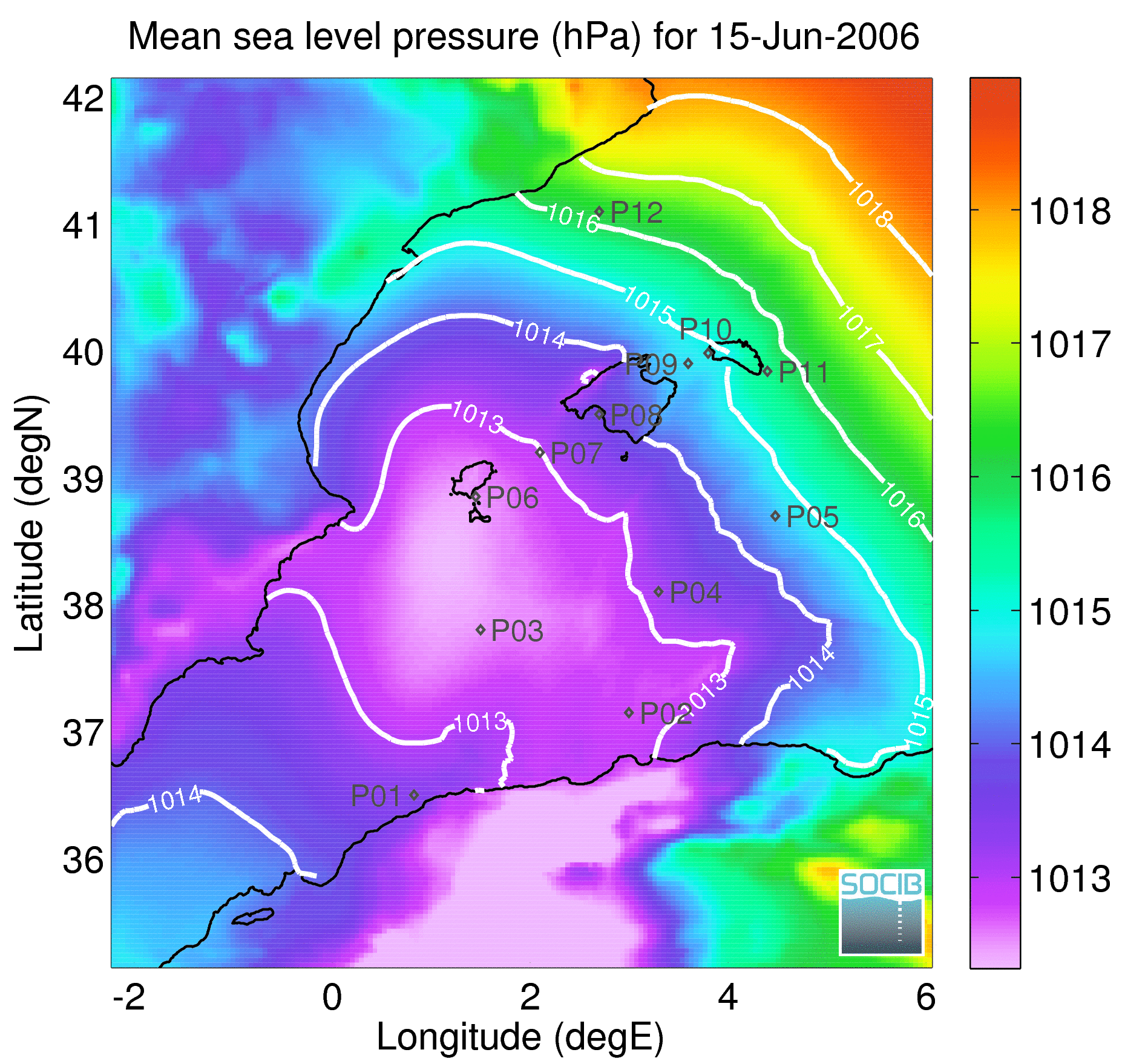
BRIFS representation of the 15 June 2006 Rissaga
|
The figure below illustrates sea level anomalies predicted in the Bay of Palma, in the middle of Menorca Channel, at the entrance of Ciutadella harbor and inside the harbour. 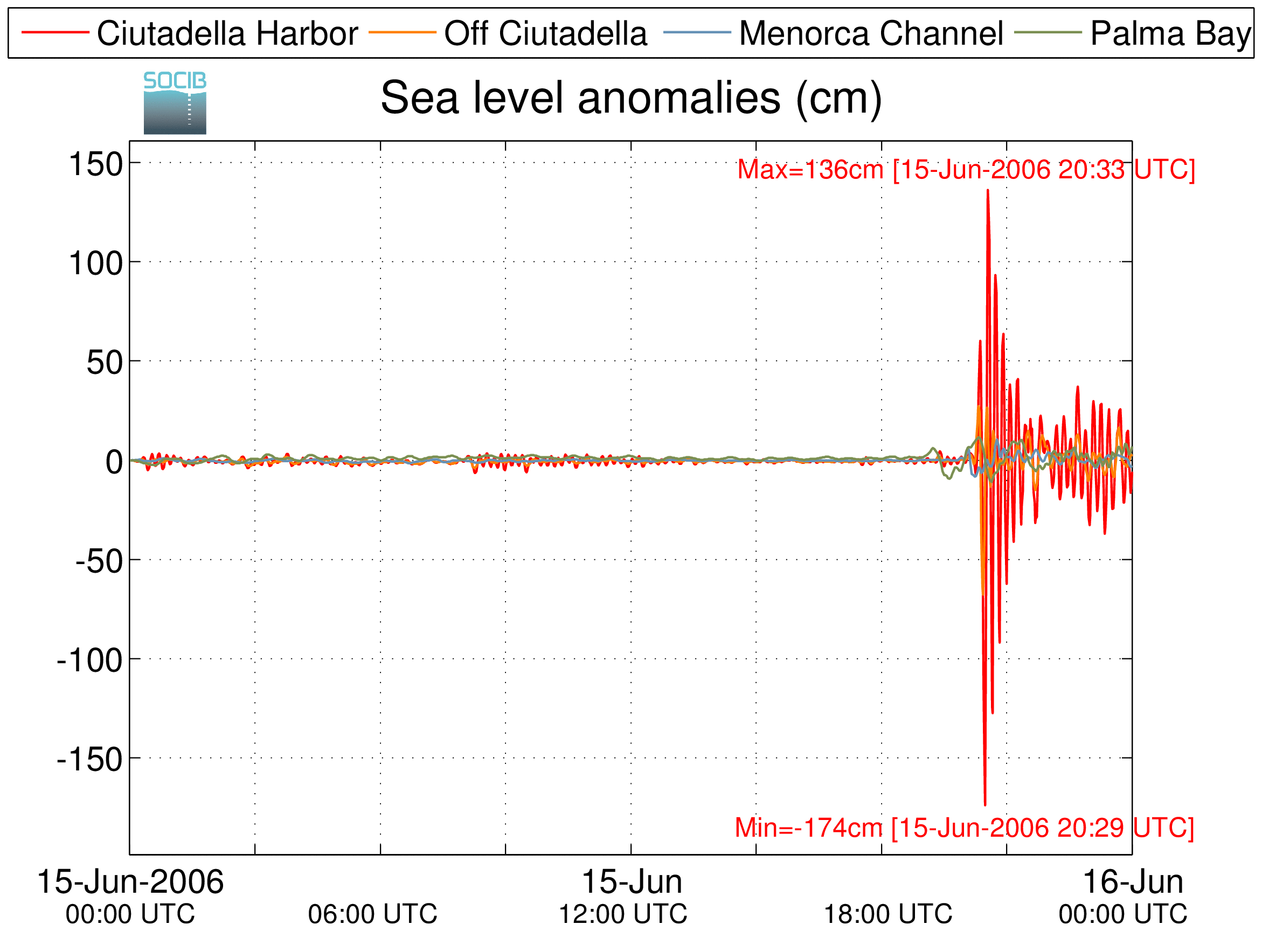
Sea level anomaly predictions |
| 0-24h prediction | 24-48h prediction |
|---|---|
| Download video | Download video |
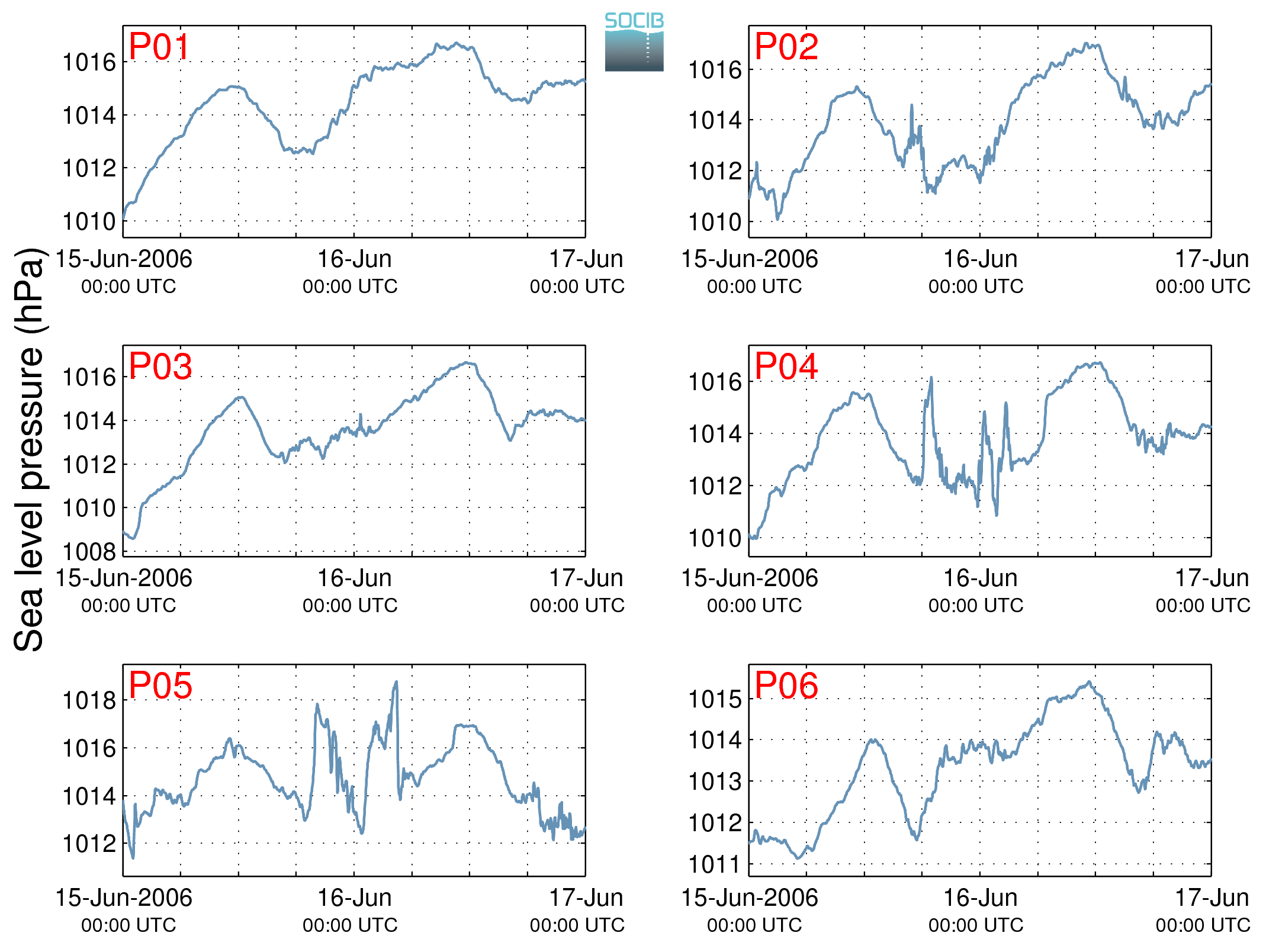
Atmospheric sea level pressure evolution at P1, P2, P3, P4, P5 and P6 |

Atmospheric sea level pressure evolution at P7, P8, P9, P10, P11 and P12 |